LLM study notes: Positional Encoding
This post is part of my study notes of LLM.
When the Transformer model was introduced in the seminal paper “Attention is All You Need”, it revolutionized the way we approach sequence-to-sequence tasks. One of the critical components of this architecture is positional encoding. This feature allows the model to understand the order of words in a sentence, which is crucial for many language-related tasks. Let’s dive into the concept of positional encoding, inspired by the PyTorch implementation.
What is Positional Encoding?
In neural networks, particularly those that deal with language, we need a way to represent words as vectors. This process is called word embedding. However, standard word embeddings don’t contain any information about the order of words — they are position-agnostic. Imagine trying to understand a sentence without knowing the sequence of words; it would be almost impossible!
Positional encoding is the solution to this problem. It adds unique information to each word embedding that indicates the word’s position in the sentence. This way, even if two sentences contain the same words, the model can distinguish them based on the order of those words.
Visualizing the Role of Positional Encoding
Let’s walk through a graphical representation:
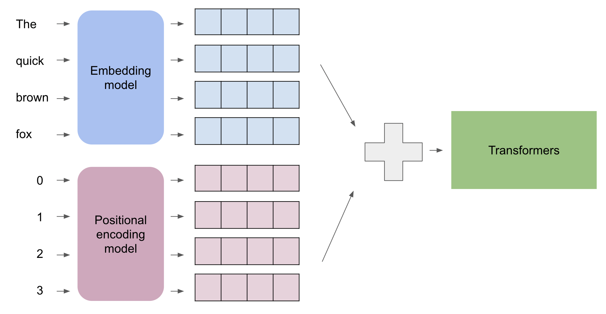
The diagram showcases the flow of information through the initial stages of a Transformer model:
- Words to Embeddings:
- On the left, we have individual words: “The,” “quick,” “brown,” and “fox.”
- These words are fed into an “Embedding model” which transforms each word into a multi-dimensional vector, represented by the blue rectangles. The size of these rectangles indicates the dimensionality of the word embeddings.
- Position to Positional Encodings:
- Parallel to the word embeddings, we have positions (0, 1, 2, and 3) corresponding to each word in the sequence. It’s crucial to note that these are not word embeddings but rather the position of the words in the sequence.
- These positions are processed by the “Positional encoding model,” producing a unique vector for each position. These are depicted by the pink rectangles. The size of the positional encoding vectors matches that of the word embeddings, allowing them to be combined.
- Combining Word Embeddings and Positional Encodings:
- The individual word embeddings and their corresponding positional encodings are then summed together. This summation embeds the positional information into the word embeddings.
- Input to Transformer:
- The resulting vectors, now enriched with positional information, are fed into the Transformer. From here, the Transformer processes the information using its multiple layers of attention mechanisms and feed-forward networks to generate outputs.
The Pytorch Implementation
import torch
import math
seq_len = 128 # number of tokens in the sequence
d_model = 8   # embedding vector length for each token
pe = torch.zeros(seq_len, d_model)
position = torch.arange(0, seq_len, dtype=torch.float).unsqueeze(1)
div_term = torch.exp(torch.arange(0, d_model, 2).float() * (-math.log(10000.0) / d_model))
pe[:, 0::2] = torch.sin(position * div_term)
pe[:, 1::2] = torch.cos(position * div_term)
pe = pe.unsqueeze(0).transpose(0, 1)
At the end of execution, pe is of shape (128, 1, 8) corresponding to sequence length, batch size, d_model, which is exactly the same shape as the word embeddings. The values of pe are in range [-1,1] so naturally scaled for any values of sequence length.
Visualizing Positional Encoding
The positional encoding function uses a combination of sine and cosine functions to generate a unique positional signal. The choice of sine and cosine functions provides a way to encode position information that is easily interpretable by the model and allows for the model to generalize to sequence lengths that it has not seen during training.
In our Python code, div_term is a crucial component that modifies the frequency of the sine and cosine functions for each element along the d_model dimension:
div_term = torch.exp(torch.arange(0, d_model, 2).float() * (-math.log(10000.0) / d_model))
div_term is a vector of shape d_model/2.
Translated to a mathematical function, this becomes:
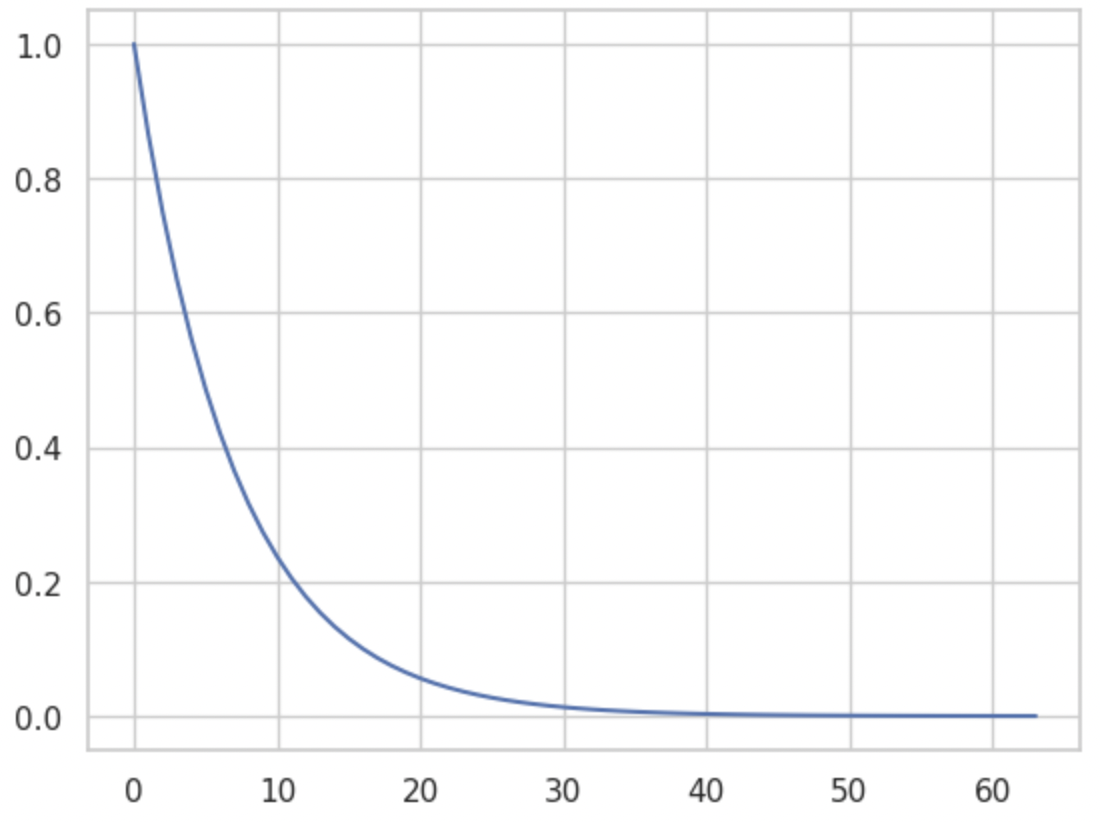
$f(x) = \exp \left( x \times \left( -\frac{\log(10000.0)}{d_{\text{model}}} \right) \right)$
Note that $-\frac{\log(10000.0)}{d_{\text{model}}}$ is a constant so essentially it is just $f(x) = \exp(xc)$. If we plot it, the function looks like this:
So essentially, with the div_term the frequency decreases along the dimention of d_model. This can be proved by drawing a heat map of pe as shown below:
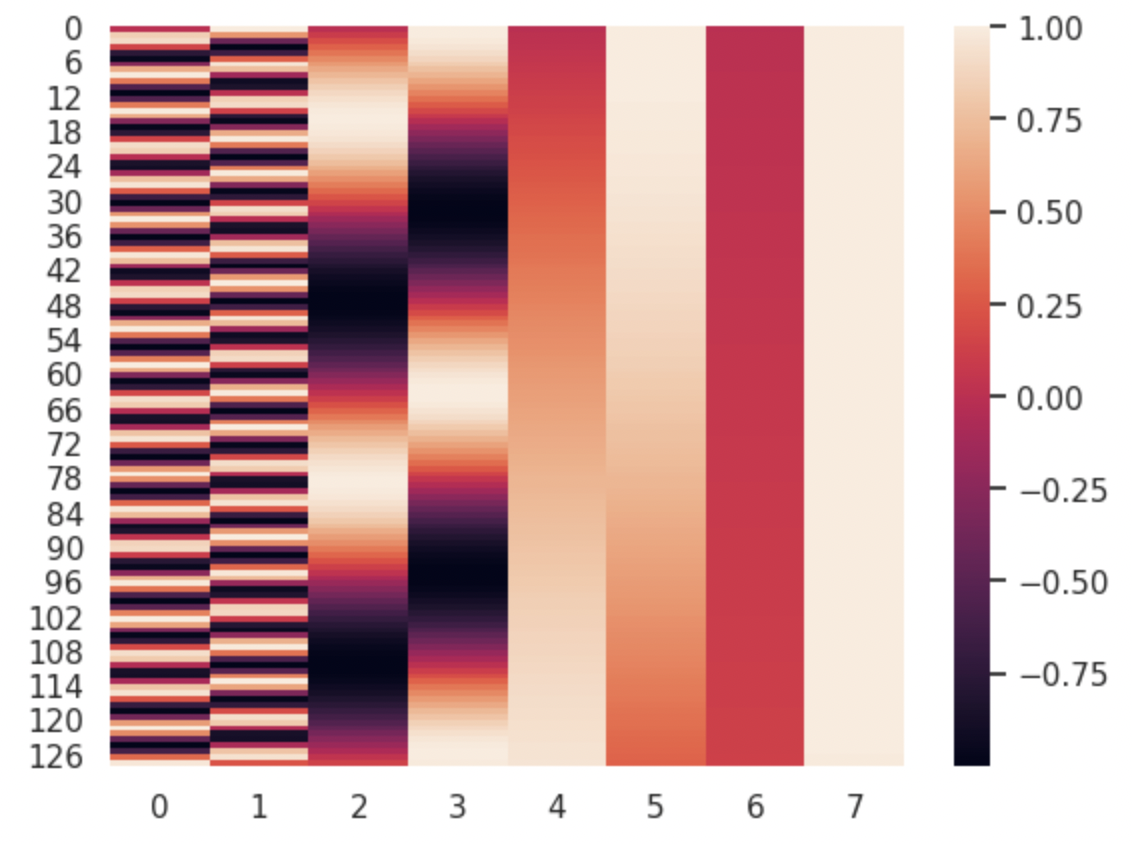
- Axes:
- The Y-axis represents the sequence length, ranging from 0 to 127 (a total of 128 positions).
- The X-axis indicates the embedding dimensions, starting from 0 to 7 (embedding size of 8).
- Color Spectrum:
- The color bar on the right denotes the values of positional encodings: darker shades of purple correspond to negative values, while shades of orange indicate positive values.
- Patterns in Heatmap:
- Columns 0 and 1: Display an alternating stripe pattern, indicating a periodicity of sinusoidal functions (like sine and cosine) for generating positional encodings. The width of the bands indicates the frequency of the oscillations.
- Columns 2 to 7: Show smoother gradients compared to the first two columns. The color shifts gradually, indicating a slower change in the value of positional encodings across these dimensions, so smaller frequency.
The diverse patterns across columns ensure that each position in the sequence has a unique encoding, helping the model to distinguish different positions.
In the heat map, each row is a vector representing each position. We can use TSNE to visualize the relationship of these vectors.
import numpy as np
from sklearn.manifold import TSNE
import matplotlib.pyplot as plt

# Assuming X is your matrix with multiple dimensions per sample
# For this example, let's create a random dataset
X = pe[:,0,:].numpy()  # 100 samples with 20 features each

# Create a t-SNE instance: you can specify the number of components (n_components),
# which is the number of dimensions you want to reduce your data to.
tsne = TSNE(n_components=2, random_state=0,perplexity=4)

# Fit and transform the data with t-SNE: this can take some time depending on your dataset size
X_tsne = tsne.fit_transform(X)

# Plotting the result of t-SNE
plt.figure(figsize=(12, 8))
for i in range(X_tsne.shape[0]):
    plt.scatter(X_tsne[i, 0], X_tsne[i, 1])
    plt.annotate(f'{i}', (X_tsne[i, 0], X_tsne[i, 1]), fontsize=9)
plt.title('t-SNE visualization of high-dimensional data')
plt.xlabel('t-SNE feature 1')
plt.ylabel('t-SNE feature 2')
plt.show()
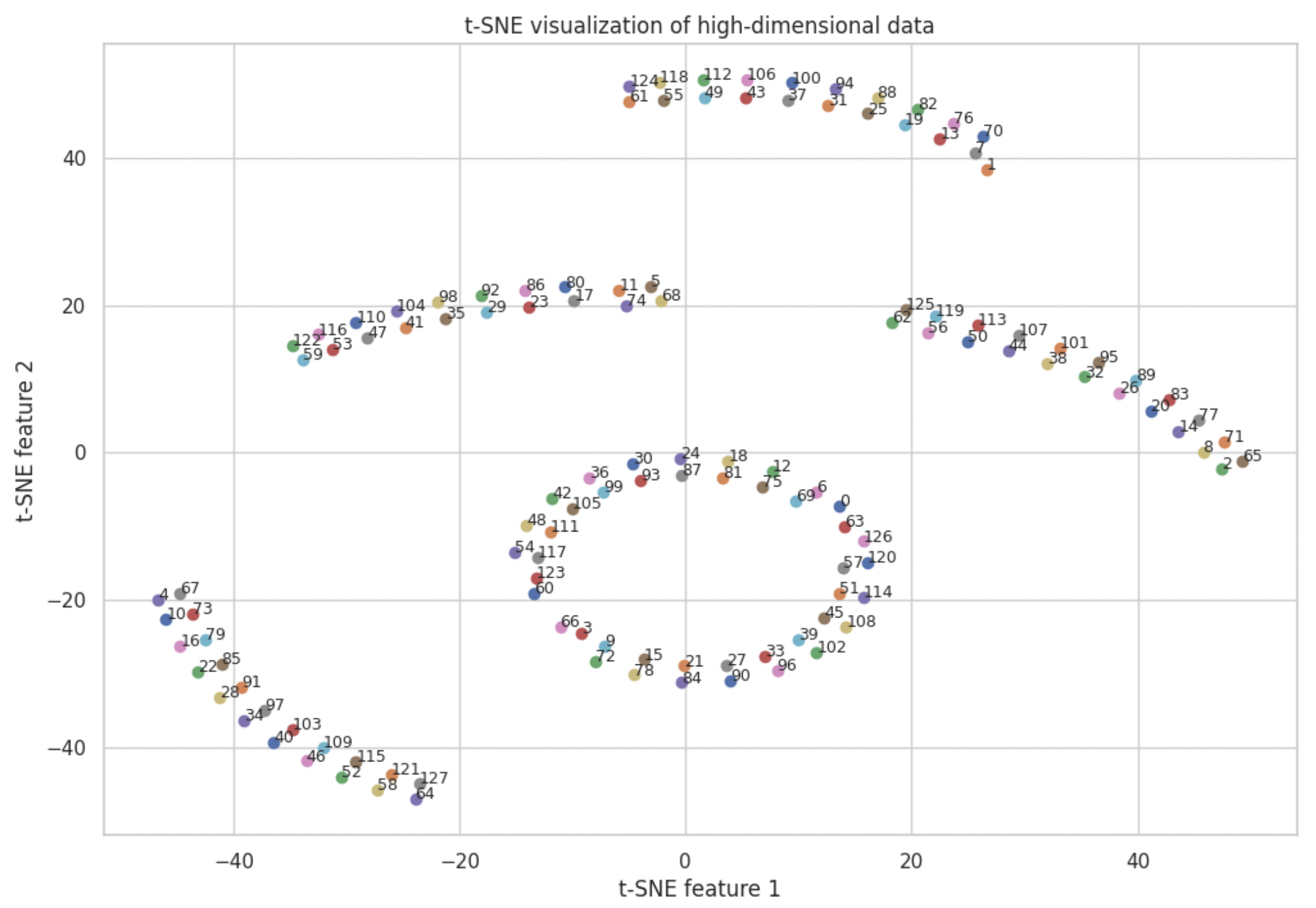
Each data point is labeled with a number, which represents a positional encoded vector for each position in the sequence (from 0 to 127). The postional encoded vectors are fairly scattered across the 2D space, which is what we want. However, there are distinct clusters. The pattern of periodicity emerges again. Looking closely at each cluster, we can see periodicity of 6 and 63. The periodicity introduces a bias to positions. For example, it is not likely that position 5 and position 68 should be that close in real world sentences. More advanced positional encoding algorithms are needed to revove such biases.
Conclusion
Positional encoding is a beautifully simple yet powerful idea that allows models to account for the order of data in sequences. As we continue to push the boundaries of what’s possible with machine learning, concepts like positional encoding remind us of the importance of incorporating human-like understanding—such as the significance of word order—into our models.